Visualization - Basic Dashboard#
The Boltzmann Wealth Model#
If you want to get straight to the tutorial checkout these environment providers:
![]() (This can take 30 seconds to 5 minutes to load)
(This can take 30 seconds to 5 minutes to load)
Due to conflict with Colab and Solara there are no colab links for this tutorial
If you are running locally, please ensure you have the latest Mesa version installed.
Tutorial Description#
This tutorial extends the Boltzmann wealth model from the AgentSet tutorial, by adding an interactive dashboard.
In this portion, we will demonstrate how users can employ build a basic dashboard. This is part one of three part series on building interactive dashboards in Mesa.
If you are starting here please see the Running Your First Model tutorial for dependency and start-up instructions
Import Dependencies#
This includes importing of dependencies needed for the tutorial.
# Has multi-dimensional arrays and matrices.
# Has a large collection of mathematical functions to operate on these arrays.
import numpy as np

# Data manipulation and analysis.
import pandas as pd

# Data visualization tools.
import seaborn as sns

import mesa
from mesa.discrete_space import CellAgent, OrthogonalMooreGrid
from mesa.visualization import SolaraViz, SpaceRenderer, make_plot_component
from mesa.visualization.components import AgentPortrayalStyle
/home/docs/checkouts/readthedocs.org/user_builds/mesa/envs/2873/lib/python3.13/site-packages/solara/validate_hooks.py:122: UserWarning: /home/docs/checkouts/readthedocs.org/user_builds/mesa/envs/2873/lib/python3.13/site-packages/mesa/visualization/solara_viz.py:399: ComponentsView: `use_state` found despite early return on line 376
To suppress this check, replace the line with:
    current_tab_index, set_current_tab_index = solara.use_state(0)  # noqa: SH101

Make sure you understand the consequences of this, by reading about the rules of hooks at:
    https://solara.dev/documentation/advanced/understanding/rules-of-hooks

  warnings.warn(str(e))
Basic Model#
The following is the basic model we will be using to build the dashboard. This is the same model seen in tutorials 0-3.
def compute_gini(model):
    agent_wealths = [agent.wealth for agent in model.agents]
    x = sorted(agent_wealths)
    N = model.num_agents
    B = sum(xi * (N - i) for i, xi in enumerate(x)) / (N * sum(x))
    return 1 + (1 / N) - 2 * B


class MoneyAgent(CellAgent):
    """An agent with fixed initial wealth."""

    def __init__(self, model, cell):
        """initialize a MoneyAgent instance.

        Args:
            model: A model instance
        """
        super().__init__(model)
        self.cell = cell
        self.wealth = 1

    def move(self):
        """Move the agent to a random neighboring cell."""
        self.cell = self.cell.neighborhood.select_random_cell()

    def give_money(self):
        """Give 1 unit of wealth to a random agent in the same cell."""
        cellmates = [a for a in self.cell.agents if a is not self]

        if cellmates:  # Only give money if there are other agents present
            other = self.random.choice(cellmates)
            other.wealth += 1
            self.wealth -= 1

    def step(self):
        """do one step of the agent."""
        self.move()
        if self.wealth > 0:
            self.give_money()


class MoneyModel(mesa.Model):
    """A model with some number of agents."""

    def __init__(self, n=10, width=10, height=10, seed=None):
        """Initialize a MoneyModel instance.

        Args:
            N: The number of agents.
            width: width of the grid.
            height: Height of the grid.
        """
        super().__init__(seed=seed)
        self.num_agents = n
        self.grid = OrthogonalMooreGrid((width, height), random=self.random)

        # Create agents
        MoneyAgent.create_agents(
            self,
            self.num_agents,
            self.random.choices(self.grid.all_cells.cells, k=self.num_agents),
        )

        self.datacollector = mesa.DataCollector(
            model_reporters={"Gini": compute_gini}, agent_reporters={"Wealth": "wealth"}
        )
        self.datacollector.collect(self)

    def step(self):
        """do one step of the model"""
        self.agents.shuffle_do("step")
        self.datacollector.collect(self)
# Lets make sure the model works
model = MoneyModel(100, 10, 10)
for _ in range(20):
model.step()
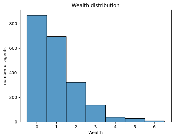
data = model.datacollector.get_agent_vars_dataframe()
# Use seaborn
g = sns.histplot(data["Wealth"], discrete=True)
g.set(title="Wealth distribution", xlabel="Wealth", ylabel="number of agents");
Adding visualization#
So far, we’ve built a model, run it, and analyzed some output afterwards. However, one of the advantages of agent-based models is that we can often watch them run step by step, potentially spotting unexpected patterns, behaviors or bugs, or developing new intuitions, hypotheses, or insights. Other times, watching a model run can explain it to an unfamiliar audience better than static explanations. Like many ABM frameworks, Mesa allows you to create an interactive visualization of the model. In this section we’ll walk through creating a visualization using built-in components, and (for advanced users) how to create a new visualization element.
First, a quick explanation of how Mesa’s interactive visualization works. The visualization is done in a browser window or Jupyter instance, using the Solara framework, a pure Python, React-style web framework. Running solara run app.py will launch a web server, which runs the model, and displays model detail at each step via a plotting library. Alternatively, you can execute everything inside a Jupyter instance and display it inline.
Grid Visualization#
Mesa’s grid visualizer works by iterating over each cell in the grid and generating a portrayal for every agent it finds. The portrayal function is called for each agent and returns an AgentPortrayalStyle—an object that defines how the agent is visually represented.
All you need to provide is a function that takes an agent as input and returns an AgentPortrayalStyle.
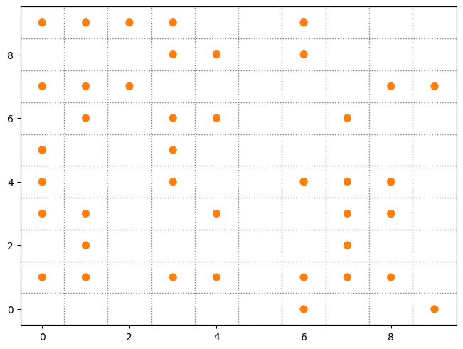
Here’s the simplest example: it draws each agent as a filled orange circle with a radius of 50.
def agent_portrayal(agent):
    return AgentPortrayalStyle(color="tab:orange", size=50)
In addition to the portrayal method, we instantiate the model parameters, some of which are modifiable by user inputs. In this case, the number of agents, N, is specified as a slider of integers.
model_params = {
    "n": {
        "type": "SliderInt",
        "value": 50,
        "label": "Number of agents:",
        "min": 10,
        "max": 100,
        "step": 1,
    },
    "width": 10,
    "height": 10,
}
Next, we instantiate the visualization object which (by default) displays the grid containing the agents, and timeseries of values computed by the model’s data collector. In this example, we specify the Gini coefficient.
There are 3 main buttons (we will discuss the play interval, render interval and use threads in lesson 6):
the step button, which advances the model by 1 step
the play button, which advances the model indefinitely until it is paused
the pause button, which pauses the model
To reset the model, the order of operations are important
Stop the model
Update the parameters (e.g. move the sliders)
Press reset
SpaceRenderer#
This is the Python object used to visualize the grid, agents, and property layers associated with the space and the model and is passed to the SolaraViz
We initialize the SpaceRenderer with a model instance (e.g., money_model in this case) and specify the rendering backend. The available backends are matplotlib(default) and altair.
Both backends can be extended using the post_process function, which can either be passed directly to the render() method or set as a property of the renderer. (We’ll cover this in more detail later.)
The method shown here is the quickest way to set up the visualization using the render() function.
It renders the space, agents, and property layers—provided that the corresponding portrayal functions are supplied for both agents and property layers.
Note:
You can make the small window full screen by clicking the button in the top-right corner of the title bar.
Page Tab View#
Plot Components#
You can place different components (except the renderer) on separate pages according to your preference. There are no restrictions on page numbering — pages do not need to be sequential or positive. Each page acts as an independent window where components may or may not exist.
The default page is page=0. If pages are not sequential (e.g., page=1 and page=10), the system will automatically create the 8 empty pages in between to maintain consistent indexing. To avoid empty pages in your dashboard, use sequential page numbers.
To assign a plot component to a specific page, pass the page keyword argument to make_plot_component. For example, the following will display the plot component on page 1:
plot_comp = make_plot_component("encoding", page=1)
Custom Components#
In tutorial 8, you will learn how to create custom components for the Solara dashboard. If you want a custom component to appear on a specific page, you must pass it as a tuple containing the component and the page number.
@solara.component
def CustomComponent():
    ...

page = SolaraViz(
    model,
    renderer,
    components=[(CustomComponent, 1)]  # Custom component will appear on page 1
)
⚠️ Warning Running the model can be performance-intensive. It is strongly recommended to pause the model in the dashboard before switching pages.
# Create initial model instance
money_model = MoneyModel(n=50, width=10, height=10)  # keyword arguments

renderer = SpaceRenderer(model=money_model, backend="matplotlib").render(
    agent_portrayal=agent_portrayal
)

GiniPlot = make_plot_component("Gini", page=1)

page = SolaraViz(
    money_model,
    renderer,
    components=[GiniPlot],
    model_params=model_params,
    name="Boltzmann Wealth Model",
)
# This is required to render the visualization in the Jupyter notebook
page
Next Steps#
Check out the next visualization tutorial dynamic agents on how to further enhance your interactive dashboard.
[Comer2014] Comer, Kenneth W. “Who Goes First? An Examination of the Impact of Activation on Outcome Behavior in AgentBased Models.” George Mason University, 2014. http://mars.gmu.edu/bitstream/handle/1920/9070/Comer_gmu_0883E_10539.pdf
[Dragulescu2002] Drăgulescu, Adrian A., and Victor M. Yakovenko. “Statistical Mechanics of Money, Income, and Wealth: A Short Survey.” arXiv Preprint Cond-mat/0211175, 2002. http://arxiv.org/abs/cond-mat/0211175.