Visualization - Custom Components#
The Boltzmann Wealth Model#
If you want to get straight to the tutorial checkout these environment providers:
![]() (This can take 30 seconds to 5 minutes to load)
(This can take 30 seconds to 5 minutes to load)
Due to conflict with Colab and Solara there are no colab links for this tutorial
If you are running locally, please ensure you have the latest Mesa version installed.
Tutorial Description#
This tutorial extends the Boltzmann wealth model from the Visualization Basic Dashboard tutorial, by adding an interactive dashboard.
In this portion, we will demonstrate how users can employ create dynamic agent representation with their Mesa dashboards. This is part two of three visualization tutorials.
If you are starting here please see the Running Your First Model tutorial for dependency and start-up instructions
Import Dependencies#
This includes importing of dependencies needed for the tutorial.
# Has multi-dimensional arrays and matrices.
# Has a large collection of mathematical functions to operate on these arrays.
import numpy as np

# Data manipulation and analysis.
import pandas as pd

# Data visualization tools.
import seaborn as sns

import mesa
from mesa.discrete_space import CellAgent, OrthogonalMooreGrid
from mesa.visualization import SolaraViz, make_plot_component, make_space_component
/home/docs/checkouts/readthedocs.org/user_builds/mesa/envs/2873/lib/python3.13/site-packages/solara/validate_hooks.py:122: UserWarning: /home/docs/checkouts/readthedocs.org/user_builds/mesa/envs/2873/lib/python3.13/site-packages/mesa/visualization/solara_viz.py:399: ComponentsView: `use_state` found despite early return on line 376
To suppress this check, replace the line with:
    current_tab_index, set_current_tab_index = solara.use_state(0)  # noqa: SH101

Make sure you understand the consequences of this, by reading about the rules of hooks at:
    https://solara.dev/documentation/advanced/understanding/rules-of-hooks

  warnings.warn(str(e))
Basic Model#
The following is the basic model we will be using to build the dashboard. This is the same model seen in tutorials 0-3.
def compute_gini(model):
    agent_wealths = [agent.wealth for agent in model.agents]
    x = sorted(agent_wealths)
    N = model.num_agents
    B = sum(xi * (N - i) for i, xi in enumerate(x)) / (N * sum(x))
    return 1 + (1 / N) - 2 * B


class MoneyAgent(CellAgent):
    """An agent with fixed initial wealth."""

    def __init__(self, model, cell):
        """initialize a MoneyAgent instance.

        Args:
            model: A model instance
        """
        super().__init__(model)
        self.cell = cell
        self.wealth = 1

    def move(self):
        """Move the agent to a random neighboring cell."""
        self.cell = self.cell.neighborhood.select_random_cell()

    def give_money(self):
        """Give 1 unit of wealth to a random agent in the same cell."""
        cellmates = [a for a in self.cell.agents if a is not self]

        if cellmates:  # Only give money if there are other agents present
            other = self.random.choice(cellmates)
            other.wealth += 1
            self.wealth -= 1

    def step(self):
        """do one step of the agent."""
        self.move()
        if self.wealth > 0:
            self.give_money()


class MoneyModel(mesa.Model):
    """A model with some number of agents."""

    def __init__(self, n=10, width=10, height=10, seed=None):
        """Initialize a MoneyModel instance.

        Args:
            N: The number of agents.
            width: width of the grid.
            height: Height of the grid.
        """
        super().__init__(seed=seed)
        self.num_agents = n
        self.grid = OrthogonalMooreGrid((width, height), random=self.random)

        # Create agents
        MoneyAgent.create_agents(
            self,
            self.num_agents,
            self.random.choices(self.grid.all_cells.cells, k=self.num_agents),
        )

        self.datacollector = mesa.DataCollector(
            model_reporters={"Gini": compute_gini}, agent_reporters={"Wealth": "wealth"}
        )
        self.datacollector.collect(self)

    def step(self):
        """do one step of the model"""
        self.agents.shuffle_do("step")
        self.datacollector.collect(self)
# Lets make sure the model works
model = MoneyModel(100, 10, 10)
for _ in range(20):
model.step()
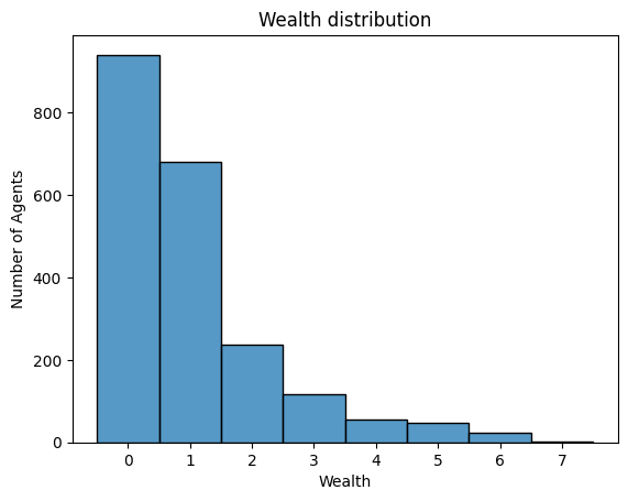
data = model.datacollector.get_agent_vars_dataframe()
# Use seaborn
g = sns.histplot(data["Wealth"], discrete=True)
g.set(title="Wealth distribution", xlabel="Wealth", ylabel="Number of Agents");
Adding visualization#
So far, we’ve built a model, run it, and analyzed some output afterwards. However, one of the advantages of agent-based models is that we can often watch them run step by step, potentially spotting unexpected patterns, behaviors or bugs, or developing new intuitions, hypotheses, or insights. Other times, watching a model run can explain it to an unfamiliar audience better than static explanations. Like many ABM frameworks, Mesa allows you to create an interactive visualization of the model. In this section we’ll walk through creating a visualization using built-in components, and (for advanced users) how to create a new visualization element.
First, a quick explanation of how Mesa’s interactive visualization works. The visualization is done in a browser window or Jupyter instance, using the Solara framework, a pure Python, React-style web framework. Running solara run app.py will launch a web server, which runs the model, and displays model detail at each step via a plotting library. Alternatively, you can execute everything inside a Jupyter instance and display it inline.
Thanks to @Corvince for all his work creating Mesa’s visualization capability
Building Custom Components#
This section is for users who have a basic familiarity with Python’s Matplotlib plotting library.
If the visualization elements provided by Mesa aren’t enough for you, you can build your own and plug them into the model server.
For this example, let’s build a simple histogram visualization, which can count the number of agents with each value of wealth.
First we need to update our imports
We use Matplotlib in this tutorial, but Mesa also has Altair. If you would like other visualization support like Plotly or Bokeh, please feel free to contribute
In addition, due to the way Solara works we need to trigger an update whenever the underlying model changes. For this you need to register an update counter with every component.
import solara
from matplotlib.figure import Figure

from mesa.visualization.utils import update_counter
Next we provide a function for our agent portrayal and our model parameters.
def agent_portrayal(agent):
    size = 10
    color = "tab:red"
    if agent.wealth > 0:
        size = 50
        color = "tab:blue"
    return {"size": size, "color": color}


model_params = {
    "n": {
        "type": "SliderInt",
        "value": 50,
        "label": "Number of agents:",
        "min": 10,
        "max": 100,
        "step": 1,
    },
    "width": 10,
    "height": 10,
}
Page Tab View#
Plot Components#
You can place different components (except the renderer) on separate pages according to your preference. There are no restrictions on page numbering — pages do not need to be sequential or positive. Each page acts as an independent window where components may or may not exist.
The default page is page=0. If pages are not sequential (e.g., page=1 and page=10), the system will automatically create the 8 empty pages in between to maintain consistent indexing. To avoid empty pages in your dashboard, use sequential page numbers.
To assign a plot component to a specific page, pass the page keyword argument to make_plot_component. For example, the following will display the plot component on page 1:
plot_comp = make_plot_component("encoding", page=1)
Custom Components#
If you want a custom component to appear on a specific page, you must pass it as a tuple containing the component and the page number.
@solara.component
def CustomComponent():
    ...

page = SolaraViz(
    model,
    renderer,
    components=[(CustomComponent, 1)]  # Custom component will appear on page 1
)
⚠️ Warning Running the model can be performance-intensive. It is strongly recommended to pause the model in the dashboard before switching pages.
Now we add our custom component. In this case we will build a histogram of agent wealth.
Besides the standard matplotlib code to build a histogram, please notice 3 key features.
@solara.componentthis is needed for any compoenent you addupdate_counter.get()this is needed so solara updates the dashboard with your agent based modelyou must initialize a
figureusing this method instead ofplt.figure(), for thread safety purpose
@solara.component
def Histogram(model):
    update_counter.get()  # This is required to update the counter
    # Note: you must initialize a figure using this method instead of
    # plt.figure(), for thread safety purpose
    fig = Figure()
    ax = fig.subplots()
    wealth_vals = [agent.wealth for agent in model.agents]
    # Note: you have to use Matplotlib's OOP API instead of plt.hist
    # because plt.hist is not thread-safe.
    ax.hist(wealth_vals, bins=10)
    solara.FigureMatplotlib(fig)
Now we create the model an initialize the visualization
# Create initial model instance
money_model = MoneyModel(n=50, width=10, height=10)

SpaceGraph = make_space_component(agent_portrayal)
GiniPlot = make_plot_component("Gini", page=1)

page = SolaraViz(
    money_model,
    components=[SpaceGraph, GiniPlot, (Histogram, 2)],
    model_params=model_params,
    name="Boltzmann Wealth Model",
)
# This is required to render the visualization in the Jupyter notebook
page
You can even run the visuals independently by calling it with the model instance
Histogram(money_model)
Exercise#
Build you own custom component
Next Steps#
Check out the next batch run tutorial on how to conduct parameter sweeps and run numerous iterations of your model.
[Comer2014] Comer, Kenneth W. “Who Goes First? An Examination of the Impact of Activation on Outcome Behavior in AgentBased Models.” George Mason University, 2014. http://mars.gmu.edu/bitstream/handle/1920/9070/Comer_gmu_0883E_10539.pdf
[Dragulescu2002] Drăgulescu, Adrian A., and Victor M. Yakovenko. “Statistical Mechanics of Money, Income, and Wealth: A Short Survey.” arXiv Preprint Cond-mat/0211175, 2002. http://arxiv.org/abs/cond-mat/0211175.